AIRI Tutorial

Imaging with AIRI

AI for Regularization in Imaging, dubbed AIRI, is a Plug-and-Play (PnP) algorithm solving inverse imaging problems in synthesis imaging by interferometry (SII) [1]. By inserting carefully trained deep neural network (DNN) as a denoiser into the proximal splitting algorithms, one waives the computational complexity of optimisation algorithms induced by sophisticated image priors, and the sub-optimality of handcrafted priors compared to Deep Neural Networks. AIRI is underpinned by the forward-backward iterative scheme. The details of AIRI are discussed in [1,2,3].

In this tutorial, we focus on a MATLAB implementation of AIRI for small-scale monochromatic intensity imaging in SII, from the environment setup, to imaging.

SII Inverse Problem

The imaging inverse problem in SII can be formulated as: \[ {\boldsymbol{y}} = {\boldsymbol{\Phi} {\boldsymbol{\bar{x}}} + \boldsymbol{n}} \] where \(\boldsymbol{y} \in \mathbb{C}^M\) is the measurement vector, \(\boldsymbol{\bar{x}} \in \mathbb{R}^N\) is the unknown radio image, \(\boldsymbol{\Phi} \in \mathbb{C}^{N \times M}\) is the measurement operator corresponding to incomplete Fourier sampling, and \(\boldsymbol{n} \in \mathbb{C}^M\) is s a realisation of a random Gaussian noise with standard deviation \(\tau\) and mean 0.

AIRI aims to recover the unknown \(\boldsymbol{\bar{x}}\) from the measurements \(\boldsymbol{y}\).

AIRI's iteration structure

AIRI is underpinned by the forward-backward (FB) algorithmic structure from optimisation theory. The FB iteration structure takes a two step-update: a forward step enforcing data fidelity, followed by a backward denoising step promoting the regularisation. \[ \boldsymbol{x}_{i+1} = \boldsymbol{\text{D}}_{\sigma} \left(\boldsymbol{x}_i - \delta \boldsymbol{\Phi}^\dagger (\boldsymbol{\Phi} \boldsymbol{x}_i - \boldsymbol{y})\right), \] where \(\boldsymbol{\Phi}^\dagger\) is the adjoint of the measurement operator. \(\boldsymbol{\text{D}}\) represents the carefully trained denoiser DNN parameterised by the noise level \(\sigma\). \(\delta > 0\) is a step size satisfying \(\delta < \frac{2}{\|\boldsymbol{\Phi}\|_S^2}\) for convergence, with \(\|\cdot\|_S\) standing for the spectral norm of its argument operator (computed using the power method). In our implementation, \(\delta\) is set to \(\delta = \frac{1.98}{\|\boldsymbol{\Phi}\|_S^2}\) (the user is not encouraged to tune this parameter).

The choice of the denoiser DNN, more specifically its noise level \(\sigma\) is crucial for best results. In fact, when \(\sigma\) is too large, the reconstructed image can be smooth. In the opposite case, it can be grainy and noisy. In [1], we proposed to build a shelf of denoiser DNNs, each trained at a fixed noise level. In imaging, the denoiser DNN is selected from the shelf whose noise level is the closest to the inverse of the estimated target image dynamic range given by: \[\sigma = \frac{\tau}{\alpha\sqrt{2\|\boldsymbol{\Phi}\|_S^2}},\] where \(\alpha\) is the maximum intensity of the target image \(\boldsymbol{\bar{x}}\). Recognising that \(\sigma\) may not fall exactly on the shelf, adequate scaling factor is applied to the denoiser's input (and its inverse is applied to the denoiser's output) to make sure the selected DNN denoiser works at its noise level. A first estimate of \(\alpha\) can be obtained from the measurements, more precisely as the peak value of the normalised back-projected data image known as the dirty image. In [3], we proposed an adaptive procedure to adjust \(\alpha\) during imaging (taken as the peak value of the image estimate) to enable the selection of the appropriate denoiser DNN from the shelf if necessary.

The above heuristic of the image-domain noise estimate which enables the selection of the appropriate DNN denoiser from the shelf has shown to be effective both in simulation [1,3] and on real data [2,3]. However, in some cases an adjustment of its value - within one order of magnitude - may be necessary for best results. The adjusting factor is by default set to 1 (i.e. adjustement is disabled) and can be fine-tuned if needed. Readers can refer to this README for more details.

Clone Repository

You can clone the repository to the current directory by running the command below.

The flag "--recurse-submodules" is required to clone the sub-module RI-measurement-operator.

Dependencies

To run the repository, your MATLAB version should be higher than R2019b. The script below looks for the required toolboxes.

Missing toolboxes can be installed from MATLAB directly. Go to the "HOME" tab of MATLAB. Then in "Add-Ons", click "Get Add-Ons" and search for the name of the missing toolbox.

Pre-trained AIRI denoisers

We provided two shelves of denoisers trained with optical astronomical image dataset (OAID shelf) and MRI dataset (MRID shelf) respectively [3]. The DNNs are in ONNX format readable in MATLAB, which can be downloaded with the commands below.

Unzip both denoiser shelves by running:

Test Dataset

For this tutorial, we provide a test dataset composed of a ground truth in .fits format and its associated measurement file in .mat format.
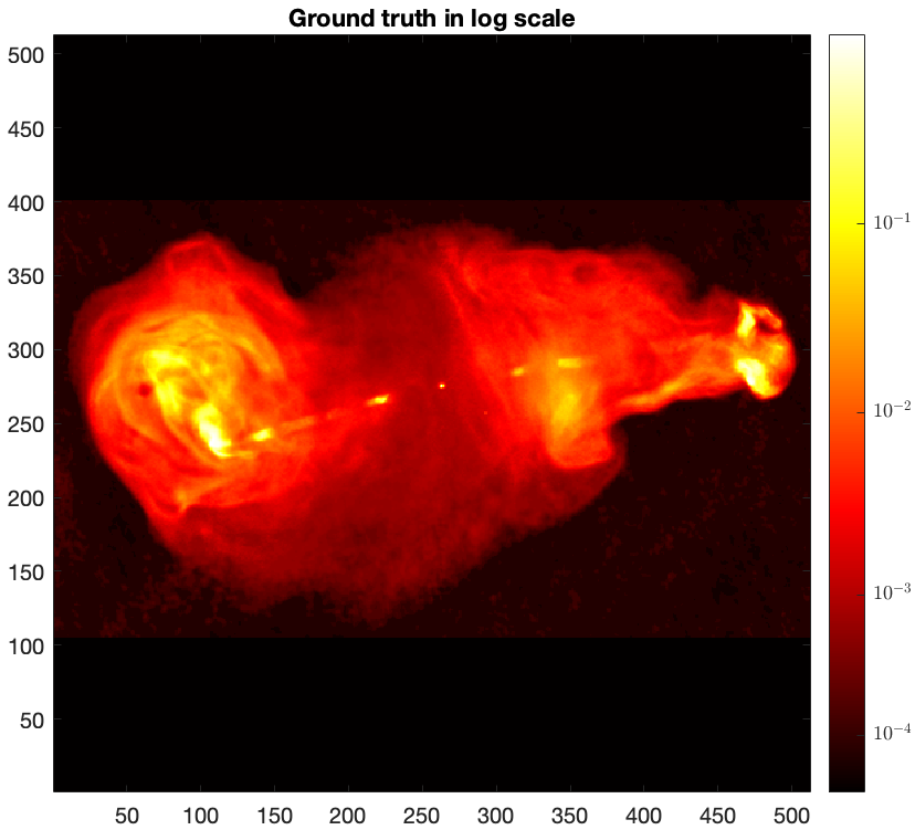
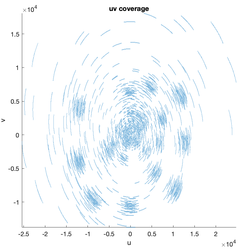
The ground truth \(\boldsymbol{\bar{x}}\) is a post-processed image of the radio galaxy 3c353 of size \(N = 512 \times 512\). The measurements are generated using a simulated Fourier sampling pattern of MeerKAT.
First, let us read and visualise the ground truth.

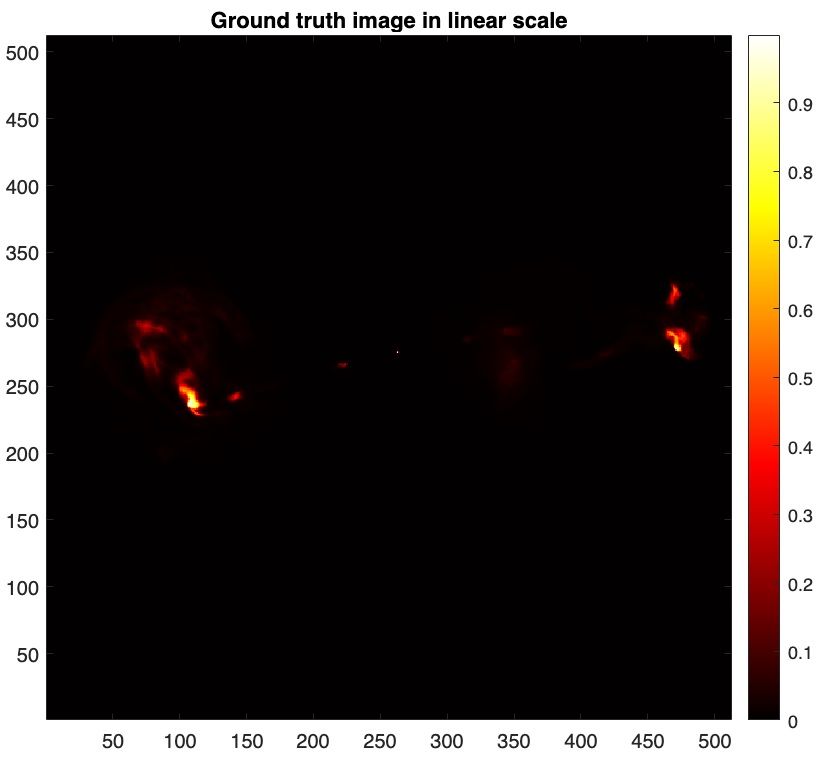
Given the large dynamic range of the ground truth, only bright features are visible in linear scale. For a better visualisation, we map its pixels intensities to the logarithmic scale using the equation below [4]: \[\textrm{rlog}(\boldsymbol{{x}}) = \boldsymbol{{x}}_{\textrm{max}} \log_{a}(\frac{a}{\boldsymbol{{x}}_{\textrm{max}}} \boldsymbol{{x}} + \boldsymbol{1}),\] where \(a>0\) and \(\boldsymbol{{x}}_{\textrm{max}}\) are the dynamic range and the maximum intensity of input image \(\boldsymbol{{x}}\) respectively. For the ground truth image \(\boldsymbol{\bar{x}}\) shown above, the maximum intensity is \(\boldsymbol{\bar{x}}_{\textrm{max}}=1\) and a dynamic range is approximately \(a=10^4\).

The test measurement file in .mat format associated with the above ground truth can be loaded via the command below.

meas = struct with fields:
           frequency: 1.0000e+09
                         y: [201600×1 double]
                         u: [201600×1 double]
                         v: [201600×1 double]
                         w: [201600×1 double]
                      nW: [201600×1 double]
              nWimag: []
maxProjBaseline: 2.5948e+04

The expected fields are listed below.

• "y", measurement/data vector.
• "u": \(\boldsymbol{u}\) coordinates in units of the observation wavelength.
• "v": \(\boldsymbol{v}\) coordinates in units of the observation wavelength.
• "w": \(\boldsymbol{w}\) coordinates in units of the observation wavelength.
• "nW": noise-whitening vector, known as the natural weights, corresponding to the inverse of the noise standard deviation. During imaging, these weights are applied to the measurements and injected into the measurement operator model.
• "nWimag": imaging weight vector, compensating for the non-uniform Fourier sampling and enhancing the effective resolution of the observations. The vector is optional and can be computed directly in the AIRI imager.
• "frequency": the observation frequency in Hz.
• "maxProjBaseline": is the maximum projected baseline in units of the observation wavelength, formally it equals to max \(\max\{\sqrt{\boldsymbol{u}^2 + \boldsymbol{v}^2}\}\). Hence, it represents the spatial bandwidth of the Fourier sampling.

The collection of the \((\boldsymbol{u}, \boldsymbol{v})\) points constitutes the 2D Fourier sampling pattern also known as the \(uv\)-coverage.

In the context of narrow-field SII, the effect of the \(\boldsymbol{w}\) coordinates is negligeable, and is therefore not considered in the measurement operator model.

Scripts to generate synthetic measurement files as well as to convert real Measurement Sets (MS) to .mat files readable by this repository are available.

Imaging with AIRI

AIRI imager is launched via the MATLAB function run_imager. This function takes as input a configuration file in .json format, where all parameters involved in the imaging process are defined and set to default values where relevant. The readers are directed to the README for more information on the content of the configuration file.

In this tutorial, we use the example configuration file ./config/AIRI_sim.json. The function run_imager also accepts optional name-argument pairs to overwrite corresponding fields in the configuration file.

The user must provide as input the target image size and the pixel size in arcsecond, either directly in the configuration file or as input argument parsed to the function run_imager. When the pixel size is not known, the user can instead specify the ratio between the spatial Fourier bandwidth of the target/ground-truth image and the bandwidth of the Fourier sampling pattern. We refer to this ratio as the superresolution factor. In such case, the pixel size in arcsecond is automatically derived from the superresolution factor as: \[\textrm{imPixelSize} = \frac{180 \times 3600}{\pi} \times \frac{1} {2 \times\textrm{maxProjBaseline} \times {\textrm{superresolution} }}\] For our test dataset, the reconstructed image size is set to \(N=512 \times 512\) same as the ground truth, and the pixel size is set such that \(\textrm{superresolution}=1.0\) (i.e. the spatial bandwidth of the Fourier sampling equals the Fourier bandwidth of the ground-truth/target image). Natural weighting is considered during imaging by default.

We use the AIRI denoiser shelf trained with optical astronomical image dataset (OAID shelf). The stopping criteria (e.g. the total number of iterations and the bound on relative variation of the estimate across the iterations) are set to default. For faster runtime, the user can consider looser values.

Under these considerations, AIRI is launched via the imaging command below. We recommend running AIRI on a machine equipped with NVIDIA GPU for MATLAB to utilise CUDA to accelerate the denoising operation. AIRI takes approximately around 20 minutes in total with CUDA acceleration.

AIRI results

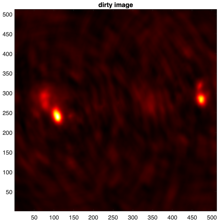
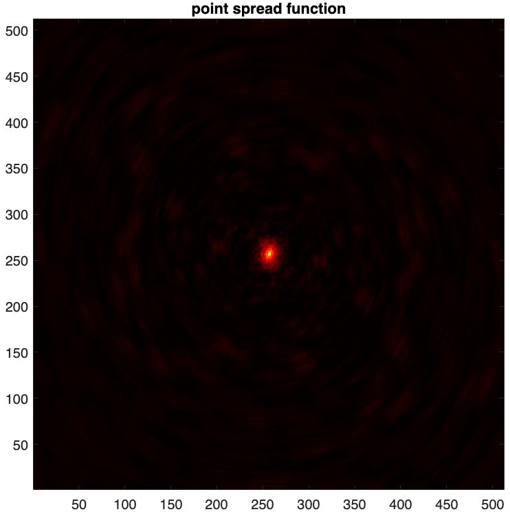
AIRI imager provides as output both the point spread function and the dirty image saved in .fits format.

• The point spread function (PSF) is defined as \(\boldsymbol{h} = \kappa\textrm{Re}\{\boldsymbol{\Phi}^{\dagger}\boldsymbol{\Phi}\boldsymbol{\delta}\}\) , with \(\boldsymbol{\delta}\) a Dirac delta image (with value 1 at its centre and 0 otherwise), and \(\kappa\) a normalisation factor ensuring its peak value is equal to 1.
• The dirty image (i.e. the normalised back-projected data) is defined as \(\boldsymbol{x}_d = \kappa \textrm{Re} \{\boldsymbol{\Phi}^{\dagger} \boldsymbol{y}\} \).

AIRI reconstructed images are saved in .fits format.

• The estimated model image \(\boldsymbol{\tilde{x}}\).
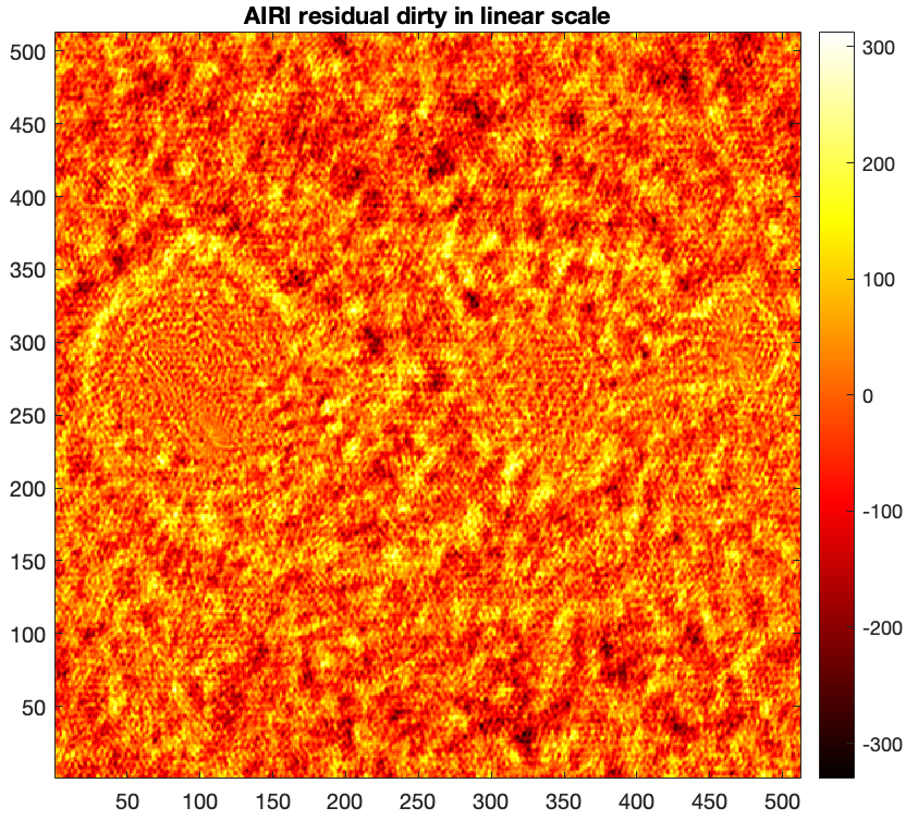
• The associated residual dirty image (i.e. normalised back-projected data residual) \(\boldsymbol{\tilde{r}} = \kappa(\textrm{Re} \{\boldsymbol{\Phi}^{\dagger} \boldsymbol{y}\} -\textrm{Re}\{\boldsymbol{\Phi}^{\dagger}\boldsymbol{\Phi} \boldsymbol{\tilde{x}}\}) \).

We assess the reconstruction quality using the two metrics below:

\[\text{SNR}(\boldsymbol{\bar{x}}, \boldsymbol{\tilde{x}}) = 20\log_{10}\left(\frac{\|\boldsymbol{\bar{x}}\|_{2}}{\|\boldsymbol{\bar{x}} - \boldsymbol{\tilde{x}}\|_{2}} \right), \]
\[ \log\text{SNR}(\boldsymbol{\bar{x}}, \boldsymbol{\tilde{x}}) = \text{SNR}(\text{rlog}(\boldsymbol{\bar{x}}), \text{rlog}(\boldsymbol{\tilde{x}})). \]

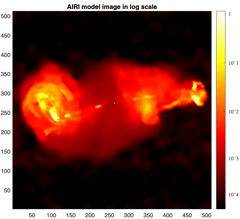
Reconstruction metrics: SNR 25.265 dB; logSNR 21.025 dB

Note that in [3], we considered a slightly different mapping of the logarithmic scale that is parameterised by the maximum intensity value \(\bar{x}_{\text{max}}\) of the ground truth and the estimate of the target dynamic range defined as \(\hat{a}=\frac{1}{\sigma},\) such that: \[\text{r}\log(\boldsymbol{x}) = \bar{x}_{\text{max}} \log_{\hat{a}} \left( \frac{\hat{a}}{\bar{x}_{\text{max}}} \cdot \boldsymbol{x} + 1 \right),\]

We report below the value of the resulting logSNR metric, to which we refer to as logSNR2.

Reconstruction metrics: logSNR2 23.381 dB

Next, we'll visualise the reconstructed image.

Additional Functionalities

The code supports data-weighting schemes during imaging (uniform or Briggs weighting). It provides the functionality to compute the imaging weights if not available in the input data file.

The repository also provides implementations of other imaging algorithms, such as cAIRI [3], uPnP-BM3D and cPnP-BM3D. We direct the readers to the full README of this repository for more information.

AIRI tutorial in MATLAB

You can download this tutorial in .mlx format and launch it directly in MATLAB .

References

[1] Terris, M., Dabbech, A., Tang, C., & Wiaux, Y., Image reconstruction algorithms in radio interferometry: From handcrafted to learned regularization denoisers. MNRAS, 518(1), 604-622, 2023.
[2] Wilber, A. G., Dabbech, A., Jackson, A., & Wiaux, Y., Scalable precision wide-field imaging in radio interferometry: I. uSARA validated on ASKAP data. MNRAS, 522(4), 5558-5575, 2023.
[3] Terris, M., Tang, C., Jackson, A., & Wiaux, Y., Plug-and-play imaging with model uncertainty quantification in radio astronomy, 2023, preprint arXiv:2312.07137.
[4] Aghabiglou, A., San Chu, C., Dabbech, A., & Wiaux, Y., The R2D2 deep neural network series paradigm for fast precision imaging in radio astronomy. ApJS, 273(1), 3, 2024.