RI Measurement Operator Tutorial

This tutorial is focused on a MATLAB implementation of the measurement operator for small-scale monochromatic intensity imaging in radio interferometry (RI). It provides detailed instructions on how to generate the measurement operator from a given Fourier sampling pattern and how to utilise it to simulate measurements.

The repository encompasses a lighter version of the NUFFT library available online and proposed by:
[1] Fessler, J. A., & Sutton, B. P., Nonuniform Fast Fourier Transforms Using Min-Max Interpolation, IEEE Trans. Image Process., 51(2), 560-574, 2003.

It also provides a w-correction functionality (via w-projection) associated with the following publication:
[2] Dabbech, A., Wolz, L., Pratley, L., McEwen, J. D., & Wiaux, Y., The w-effect in interferometric imaging: from a fast sparse measurement operator to superresolution, MNRAS, 471(4), 4300-4313, 2017.

The library is a core dependency of the Faceted-HyperSARA software for wideband RI, associated with the following publications:
[3] Thouvenin, P.-A., Abdulaziz, A. , Dabbech, A. , Repetti, A., & Wiaux, Y., Parallel faceted imaging in radio interferometry via proximal splitting (Faceted HyperSARA): I. Algorithm and simulations, MNRAS, 521(1), 1–19, 2023.
[4] Thouvenin, P.-A., Dabbech, A., Jiang, M., Thiran, J.-P., Jackson, A., & Wiaux, Y., Parallel faceted imaging in radio interferometry via proximal splitting (Faceted HyperSARA): II. Real data proof-of-concept and code , MNRAS, 521(1), 20–34, 2023.

RI Inverse Problem

Assuming a narrow field of view and in absence of direction dependent effects, at a given time instant, each pair of antennas acquires a noisy complex measurement, termed visibility, corresponding to a Fourier component of the sought radio emission. The collection of the sensed Fourier modes accumulated over the total observation period forms the Fourier sampling pattern, describing an incomplete coverage of the 2D Fourier plane.

Under these considerations, the measurement operator model reduces to a Fourier sampling operator which reads [1]: \[\boldsymbol{\Phi} = \mathbf{G}\mathbf{F}\mathbf{Z},\] where \(\boldsymbol{\Phi} \in \mathbb{C}^{N \times M}\) is the measurement operator corresponding to the non-uniform Fourier transform (NUFFT), \(M\) is the number of measurements, and \(N\) is the image dimension (i.e. number of pixels). \(\mathbf{G} \in \mathbb{C}^{M \times P}\) is a sparse interpolation matrix whose rows are convolutional kernels centered at the associated Fourier modes (i.e. \(uv\) points), \(\mathbf{F} \in \mathbb{C}^{P \times P}\) is the 2D Discrete Fourier Transform, and \(\mathbf{Z} \in \mathbb{C}^{P \times N}\) is a zero-padding operator which also incorporates the correction for the convolution performed through the de-gridding matrix \(\mathbf{G}\).

Clone Repository

You can clone the repository to the current directory by running the command below in MATLAB:

!git clone https://github.com/basp-group/RI-measurement-operator.git
cd ./RI-measurement-operator

Generate RI Measurement Operator

To start with, set up the following paths so that MATLAB can find the required functions and input files.

addpath data;
addpath nufft;
addpath lib/operators;
addpath lib/utils;
addpath lib/ddes_utils;

We will use a simulated Fourier sampling pattern generated with the VLA, provided in "tests/test.mat". It contains the \(uvw\) coordinates in meters and the observation frequency in Hz. Load the variables of interest.

myuvwdatafile = fullfile("tests","test.mat");
frequency = load(myuvwdatafile,'frequency').frequency;
u_meter = load(myuvwdatafile,'u').u;
v_meter = load(myuvwdatafile,'v').v;
w_meter = load(myuvwdatafile,'w').w;

Convert the \(uvw\) coordinates in the unit of the observation wavelength as follows (this is needed for the computation of the pixel size in physical units).

speedOfLight = 299792458; % speed of light
wavelength = speedOfLight/frequency; % observation wavelength
% convert the \(uvw\) coordinates in the units of the wavelength
u = u_meter(:) ./ wavelength;
v = v_meter(:) ./ wavelength;
w = w_meter(:) ./ wavelength;

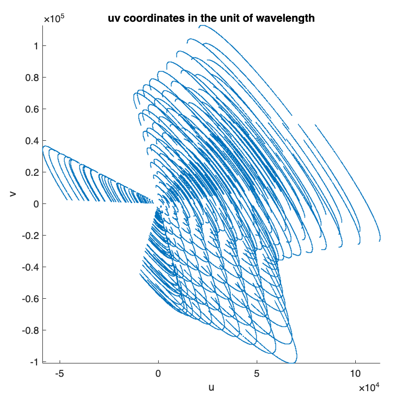
The 2D Fourier sampling pattern is described by the \(uv\) coordinates.

% plot the 2D Fourier sampling pattern
figure;
scatter(u, v, 0.1)
axis equal, axis square, axis tight
xlabel('u')
ylabel('v')
title("uv coordinates in the unit of wavelength")

To generate the measurement operator, two crucial parameters need to be set:

the ground-truth/target image dimension \(N\),
the ratio between the spatial bandwidth of the ground-truth/target image and the bandwidth of the Fourier sampling, to which we refer to as the super-resolution factor \(\textrm{superresolution} \ge 1\). The bandwidth of the Fourier sampling is given by the maximum projected baseline \(\textrm{maxProjBaseline} = \textrm{max}(\sqrt{\boldsymbol{u}^2+\boldsymbol{v}^2})\).

Note that from the value of \(\textrm{superresolution}\), one can compute the resulting pixel size of the ground-truth/target image in \(\boldsymbol{\textrm{arcsec}}\): \[\textrm{imPixelSize} = \frac{180 \times 3600}{\pi} \times \frac{1} {2 \times\textrm{maxProjBaseline} \times {\textrm{superresolution} }}\] Consider a ground-truth/target image \(\boldsymbol{\bar{x}}\) of size \(N=512 \times 512\). For the sake of this demonstration, we consider \(\textrm{superresolution}=1.5\), which means that the spatial bandwidth of the Fourier sampling corresponds to 2/3 the spatial Fourier bandwidth of the ground-truth/target image.

imSize = [512, 512]; % image size: N = 512x512
resolution_param.superresolution = 1.5; % superresolution factor
resolution_param.pixelSize = []; % pixel size in arcsec if known; keep empty to use superresolution factor instead

The measurement operator \(\boldsymbol{\Phi}\) and its adjoint \(\boldsymbol{\Phi}^\dagger\) can be generated as function handles by calling the function ops_raw_measop.m.

[measop, adjoint_measop, ~] = ops_raw_measop(u, v, w, imSize,resolution_param);

Note that, the user can input additional parameters to the function ops_raw_measop.m as shown below. Default values will be used otherwise.

% NUFFT parameters
nufft_param.N = imSize; % image size
nufft_param.J = [7, 7]; % NUFFT convolutional kernel size
nufft_param.K = 2 * imSize; % Fourier space size, with zero-padding factor 2 in each dimension
nufft_param.nshift = imSize / 2; % Fourier shift (matlab convention)
nufft_param.ktype = 'minmax:kb'; % NUFFT convolutional kernel type
% Compute data weights (e.g., uniform; Briggs)
weighting_param.gen_weights = false;
% Apply w-correction (not required for narrow fields of view)
wproj_param.enable_wproj = false;
[measop, adjoint_measop, ~] = ops_raw_measop(u, v, w, imSize, resolution_param, ...
     weighting_param, nufft_param, wproj_param);

Simulate RI measurements

To simulate RI measurements, we take a post-processed image of the radio galaxy 3c353 as the ground truth \(\boldsymbol{\bar{x}}\). The image is in .fits format provided in "tests/3c353_gdth.fits".

img_gdth = fitsread(fullfile("tests","3c353_gdth.fits")); % read the fits file
figure
imagesc(img_gdth)
colorbar, axis image, colormap('hot')
title("Ground truth image in linear scale")

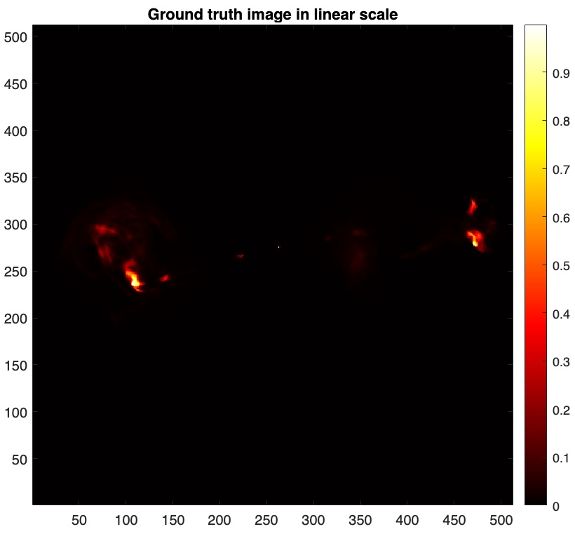
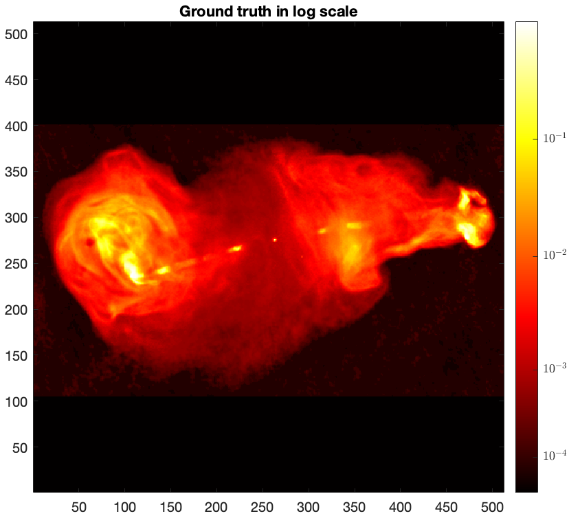
figure
imagesc(log10(img_gdth),[-4 -1]),
axis image, colorbar, colormap('hot')
title('Ground truth in log scale')

The clean visibilities are modelled as \(\boldsymbol{y}_{\textrm{clean}} = \boldsymbol{\Phi}\boldsymbol{\bar{x}}\).

y_clean = measop(img_gdth);

RI measurements modelled as \({\boldsymbol{y}} = {\boldsymbol{\Phi} {\boldsymbol{\bar{x}}} + \boldsymbol{n}}\) are subsequently obtained by adding a realisation of a white Gaussian noise \(\boldsymbol{n}\), with mean 0 and a standard deviation \(\tau\), to the clean visibilities \(\boldsymbol{y}_{\textrm{clean}} \). The value of \(\tau\) can be derived from a user-specfied input signal to noise ratio. Note that \(\tau\) can also be set to be commensurate with the dynamic range of the ground-truth image. We refer the reader to the script example_sim_ri_data.m for details.

iSNR = 40; % user-specified input SNR
M = numel(y_clean);
tau = 10^(-iSNR/20) * norm(y_clean) / sqrt(M); % calculate tau
noise = (randn(M,1) + 1i * randn(M,1)) * tau./sqrt(2); % random Gaussian noise with std tau and mean 0
y = y_clean + noise; % noisy measurements

To image the simulated RI measurements, create the associated measurement file in .mat format, that is input to the RI algorithms for small-scale monochromatic intensity imaging provided in BASPLib as shown below.

nW = ones(size(y)) ./ tau; % the inverse of the noise std
maxProjBaseline = sqrt(max(u.^2 + v.^2)); % bandwidth of the spatial Fourier sampling
save("3c353_mysimdata.mat", 'y','u','v','w','frequency','nW','-v7.3')
fprintf('\nMeasurement file saved.\n')

Imaging weighting schemes

During imaging, a common practice is to apply a whitening operation to the measurements via point-wise multiplication with the inverse of the noise standard deviation. This is known as natural weighting.

The natural weighting vector nW in our example is given by:

nW = ones(size(y)) ./ tau;

Often, this is done in combination with an additional imaging weighting scheme to compensate for the unbalance of the Fourier sampling such as uniform weighting or Briggs weighting and consequently enhance the effective resolution of the reconstruction.

The function ops_raw_measop.m enables computing these imaging weighting schemes (see the function util_gen_imaging_weights.m for details). The final weighting vector is the product of the two.

In this example, we consider Briggs weighting with robust parameter 0.

weighting_param.gen_weights = true;
weighting_param.weight_type = 'briggs'; % can be chosen from 'briggs' or 'uniform'
weighting_param.weight_robustness = 0.0; % associated with Briggs weighting

[~, ~, nWimag] = ops_raw_measop(u, v, w, imSize, resolution_param, weighting_param);

During imaging, the final weighting vector is applied to the RI measurements and is also included in the associated imaging measurement operator.

y_weighted = y .* (nW .* nWimag); % weighted data 
measop_weighted = @(x) (nW .* nWimag).* measop(x); % weighted meas. op. for imaging
adjoint_measop_weighted = @(y) adjoint_measop((nW .* nWimag) .*y); % the adjoint of the weighted meas. op. for imaging

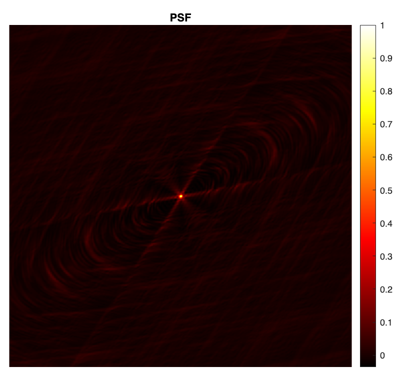
PSF & Dirty image

The point spread function (PSF) is defined as \(\boldsymbol{h} = \kappa\textrm{Re}\{\boldsymbol{\Phi}^{\dagger} \boldsymbol{\Phi}\boldsymbol{\delta}\}\), with \(\boldsymbol{\delta}\) a Dirac delta image (with value 1 at its center and 0 otherwise), and \(\kappa\) a normalisation factor ensuring that its peak value is equal to 1.

dirac = sparse(floor(imSize(1)./2)+1, floor(imSize(2)./2)+1, 1, imSize(1), imSize(2));
psf_0 = real(adjoint_measop(measop(full(dirac))));
kappa = 1./max(psf_0, [], 'all'); % normalisation factor
psf = kappa * psf_0; % normalised psf
figure
imagesc(psf)
axis square, axis off
colormap('hot')
colorbar
title("PSF")

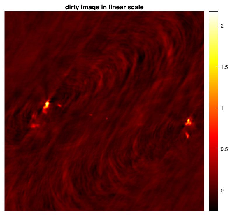
The normalised back-projected data also known as the dirty image is defined as \(\boldsymbol{x}_d = \kappa \textrm{Re} \{\boldsymbol{\Phi}^{\dagger} \boldsymbol{y}\} \).

dirty = kappa * real(adjoint_measop_weighted(y_weighted)); % the dirty image
figure
imagesc(dirty)
axis square, axis off
colormap('hot')
colorbar
title("dirty image in linear scale")

%% save PSF & dirty image
% fitswrite(dirty,'3c353_dirty.fits')
% fitswrite(psf,'psf.fits')

RI measurement operator tutorial in MATLAB

You can download this tutorial in .mlx format and launch it directly in MATLAB .